What 426 bands found in the Palisades burn scar

In January 2025 the Palisades Fire burned 23,448 acres of the Santa Monica Mountains. Planet’s Tanager-1 satellite imaged the area on 15 December, before the fire, and again on 23 January, after it was out. The animation above cuts between those two dates.

The yellow outline is the official fire perimeter from the NIFC interagency service. I pulled it in separately and dropped it on top, and the burn scar sits inside it almost exactly. On dNBR, the standard burn index, the median land pixel inside the perimeter is 0.588. Outside every mapped fire perimeter in the scene, it’s 0.060.

Any satellite with a near-infrared and a shortwave-infrared band could make that map. I spent the last few months working with Tanager because it records a lot more than that, and I wanted to know two things: what extra you can measure on a burned hillside when every pixel has a full spectrum, and how you’d check that those measurements hold up. This post covers the first set of results.

426 bands per pixel

A phone camera records three values per pixel. Sentinel-2, the free ESA mission most of us in remote sensing use daily, records 13, and about 10 of those do the work over land. Tanager-1 records 426, spaced roughly 5 nm apart from about 380 to 2,500 nm. That runs from visible light well into the shortwave infrared. The bands sit side by side, so every 30 m pixel comes with a continuous reflectance curve.

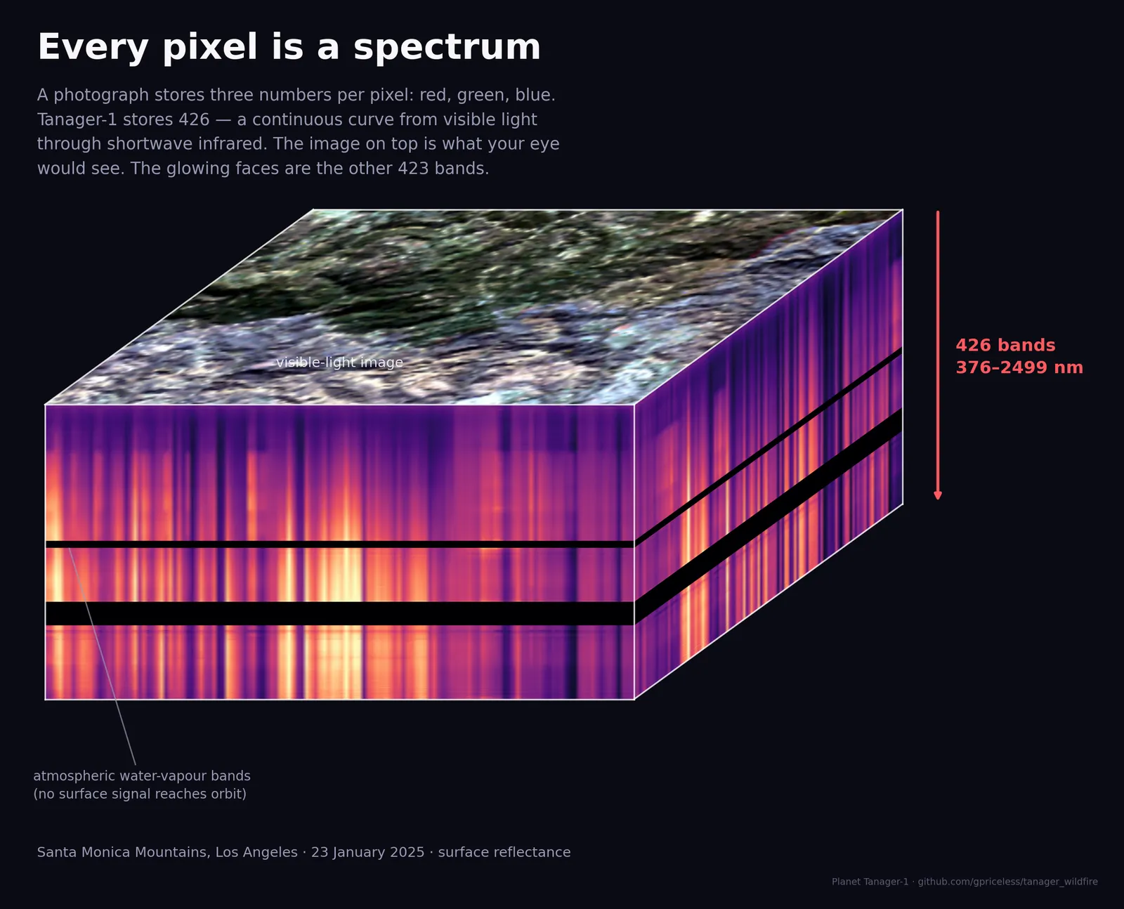
The top of the cube is a true-colour image of the scene. The sides show all 426 bands along the cube’s edges. The two black stripes are the water-vapour absorption bands around 1,400 and 1,900 nm. There, the atmosphere soaks up nearly everything and almost no light from the ground reaches the sensor. I left them black, since interpolating across them would just be inventing data.

The extra bands are useful because different surfaces have differently shaped curves.

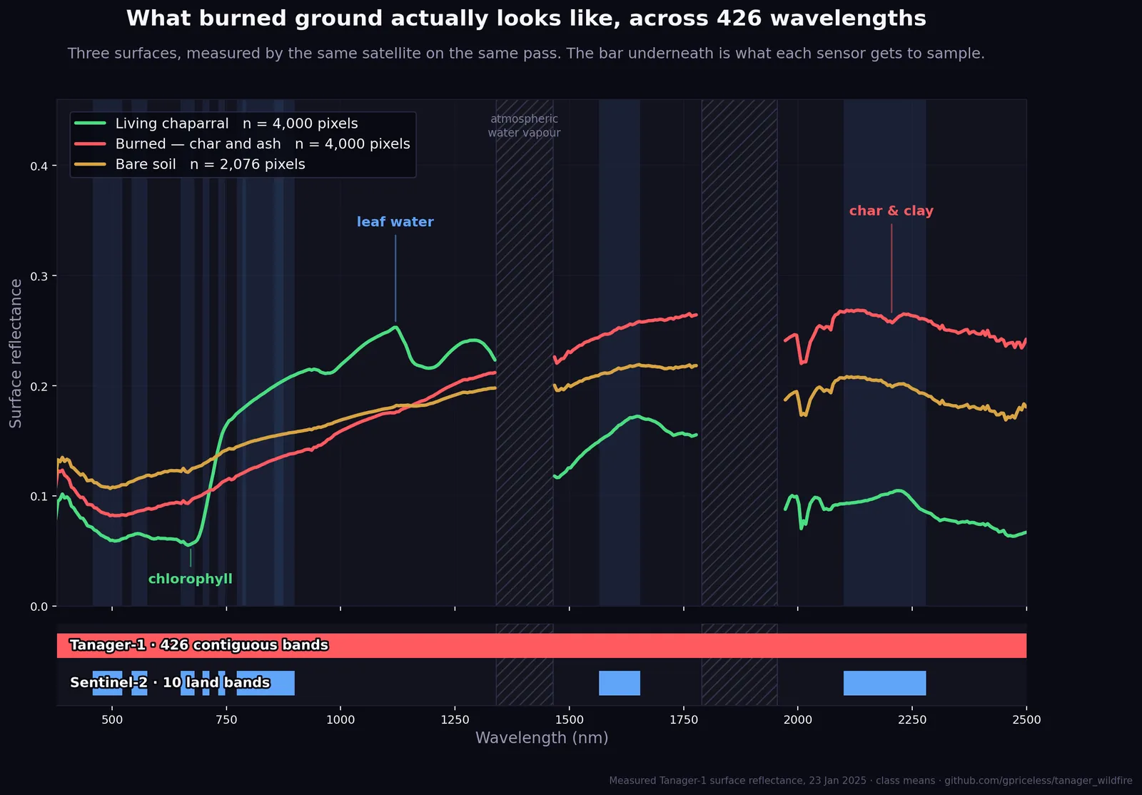
Each line averages a few thousand pixels from this scene:

• Living chaparral. A dip at 672 nm where chlorophyll absorbs red light, a sharp jump at the red edge as leaf structure scatters near-infrared back out, then dips at the water absorption features further along.
• Burned ground. Dark and flat through the visible, then a steady climb through the shortwave infrared, ending up brighter than the vegetation past about 1,500 nm.
• Bare soil. A smooth rise from one end to the other.

The bar underneath shows Tanager’s coverage as one continuous span and Sentinel-2’s as ten separate blocks. Whatever happens in the gaps between those blocks, Sentinel-2 doesn’t record. That becomes important in the third post of this series.

Three renderings of one capture

With all 426 bands on disk, you pick how to display them after the fact.

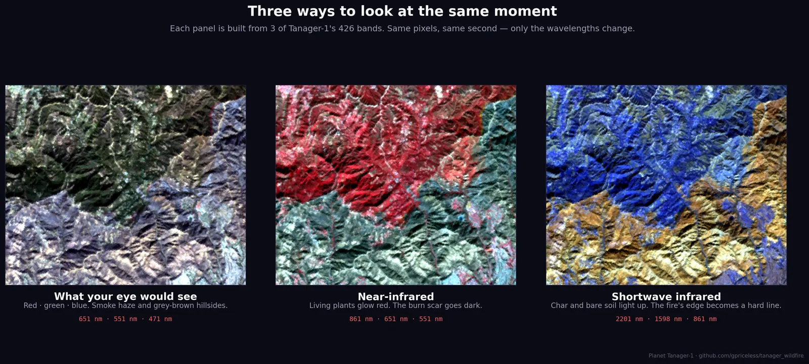
Each panel uses three bands from the same capture:

• Natural colour. The burn shows up as a grey-brown smear.
• Near-infrared. Healthy vegetation lights up red and the scar goes dark.
• Shortwave infrared. The fire edge is sharpest here, because this is where burned ground gets brighter than vegetation (the crossover in the chart above).

Each panel uses less than one percent of the data. The analysis below uses all of it.

Spectral unmixing

After a fire, a 30 m pixel on a chaparral slope holds a mix of char, surviving shrubs, dead grass and bare soil. The sensor records one blended spectrum for all of it. dNBR boils that blend down to one number for how much darker the pixel got. A pixel that’s half char and half untouched shrub can score the same as one that’s lightly scorched all over.

Spectral unmixing works backwards from the blend. You start with reference spectra for each pure material, called endmembers. Then, for each pixel, you solve for the proportions that best reproduce the spectrum the sensor measured. I used MESMA (Multiple Endmember Spectral Mixture Analysis), which tries several candidate spectra per material and keeps the best-fitting combination. There are 426 bands to fit and only four materials to solve for, so the problem is heavily over-determined. The output is four fraction maps: char, green vegetation, dry vegetation and soil.

On the Palisades scene the fits are tight, with a median error under 1% reflectance. Pixels that no combination fits well get left blank. After masking cloud, water and the edges of the swath, about 85% of the remaining land pixels get a result.

A tight fit only means the maths converged. Whether the fractions are right depends on where the reference spectra came from.

Where the endmembers came from

My first pass did what a lot of image-based workflows do and built the endmembers from the scene itself. The char endmember was the average spectrum of every pixel with NBR below −0.1 and NDVI below 0.2. So it was made of the pixels that already looked burned. Then I unmixed the scene and mapped where the char was.

You can probably see where this goes. Since char was defined as “pixels that look burned”, the char map reported where the pixels that look burned were. That’s the original threshold handed back with extra steps. Comparing that map to the fire perimeter tested nothing, because the map had no way to disagree with the assumption it was built on. The scores looked great, and they meant very little.

The second pass uses a library that never touched the image. All 23 reference spectra come from the USGS Spectral Library Version 7, measured in the field or lab years before this fire:

• 2 char spectra from a burned-area survey
• 13 shrub and tree spectra from a California field campaign, including chamise, buckbrush, manzanita, toyon and scrub oak, which cover most of these hills
• 4 cured grass spectra
• 4 bare surfaces: sand, dry playa mud and basalt

The only thing taken from the scene is the instrument’s band centres and widths, which are needed to resample the lab spectra to what Tanager would record. The script reads those two arrays and closes the file before it builds anything, so no pixel values make it into the library. The library has no idea where anything burned. If the char lands inside the fire perimeter, the method found it there.

The weak spot is soil. None of those four bare surfaces is a California soil, so I’d give the soil fraction less weight than the other three.

Results

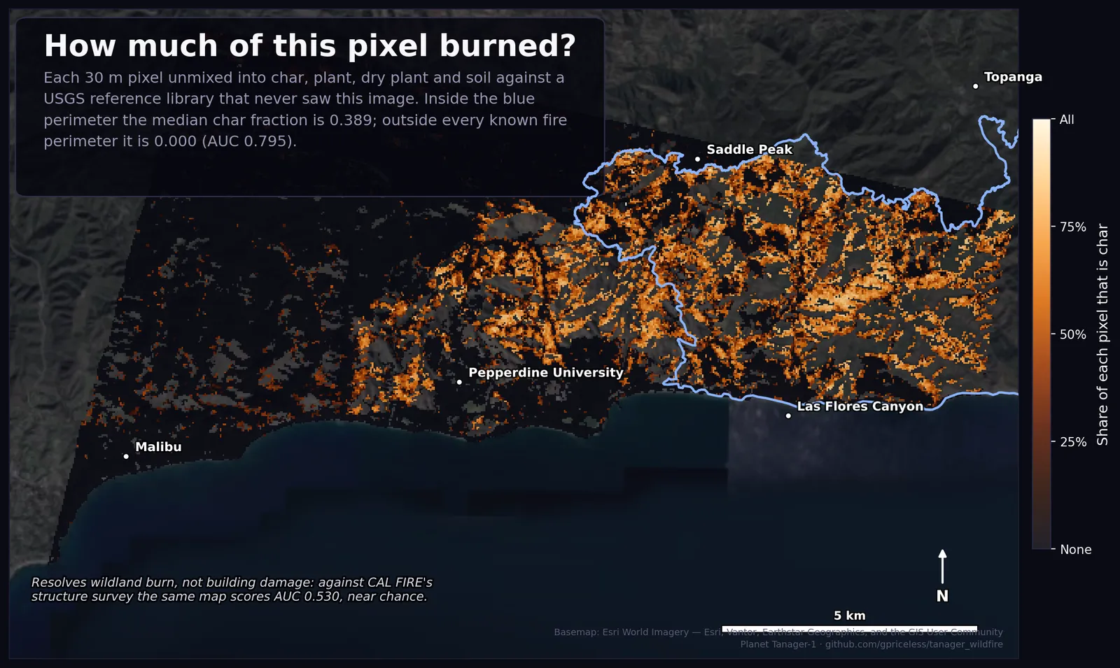
Inside the official Palisades perimeter, the median pixel is 38.9% char. Outside every known fire perimeter in the scene, the median is zero.

Separating inside from outside, the char fraction scores an AUC of 0.795. Roughly speaking, if you pick one random pixel from inside the perimeter and one from outside, the inside pixel has more char about 80% of the time. Part of the remainder is the perimeter itself. It’s a single polygon drawn around the whole event, and fires leave plenty of unburned patches inside it. The rest is the model missing.

For scale: plain dNBR, on the part of the scene where both dates overlap, scores 0.970 on the same test. The standard index is the better burn detector, comfortably. The interesting result is that a library with no knowledge of this fire found most of it anyway, and can say how much of each pixel burned.

The library also found char in two places I hadn’t asked about:

• West of the Palisades outline. This patch is the Franklin Fire, which burned Malibu Canyon in December 2024.
• North of both. About 1.4 km² of char sat in ground I’d been using as my unburned reference. I had a bad feeling about this one until I went back to the perimeter database and found the Kenneth Fire, which started on 9 January 2025 and burned 999 acres. It was in the records the whole time; I’d left it out of my query.

Fire	Median char fraction inside perimeter
Palisades	0.389
Franklin	0.337
Kenneth	0.575
Outside all three	0.000

So the evaluation had an error built into it, a burned area labelled as unburned, and the unmixing flagged it. Kenneth is now in the perimeter list, and every number above includes it. An image-derived library couldn’t have caught this, since it only knows what its threshold told it.

What this gives you

The char fraction is an estimate of how much of each wildland pixel is burned vegetation, made without field data or hand-tuned thresholds. It’s meant to sit next to dNBR in the same GIS. dNBR says how much darker a pixel got; the char fraction says what share of it is now burned material. I haven’t yet tested it against field measurements of burn severity, only against where the fire was.

It turns out to be close to useless for damaged homes. Against CAL FIRE’s structure damage survey, the same map does barely better than a coin flip. The next post covers why, plus a few other things the data couldn’t answer and some mistakes I made along the way.

Code, data and figures: FireSpec on GitHub. Imagery from Planet’s Tanager Open Data programme. Basemap: Esri World Imagery.

All writing